Markets
The markets page allows you to change how the simulation models inflation, the stock market, dividends and bonds.
Each month, the simulation randomly decides how the external markets behave. Each variable is modeled differently, but they all have a random component to model the uncertainty of the real world. By randomly modeling the markets thousands of times, the simulation hopes to provide an accurate portrayal of possible futures.
Note: You don’t have to make any changes to the default values. I’ve picked values so that the simulation will behave like the markets have behaved over the last 30 years.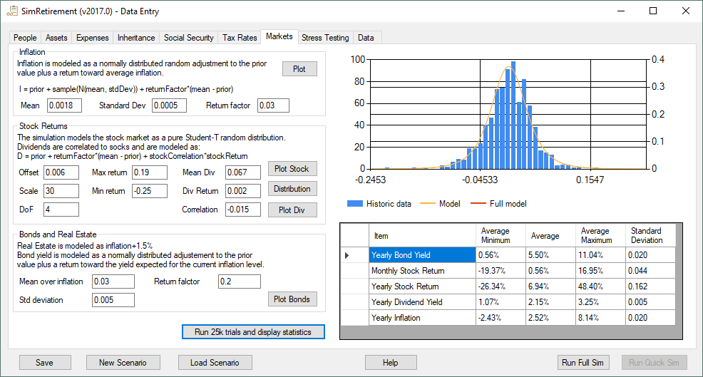
Inflation
Inflation determines how much the price of goods and services increases each month. High inflation and low stock market returns are the biggest risk factors for an early retirement. High inflation means that expenses go up quickly while the savings being used to pay those expenses is fixed. Since 1950, inflation has averaged 3.54% while for the last 20 years inflation has averaged 2.16%.
Each month, the simulation chooses a value for inflation and applies that inflation to all your expenses, the tax brackets, social security payments and any assets with the growth type of “Inflation adjusted”. The value of inflation experienced each month is not completely random. Instead it is very strongly correlated with last month’s inflation. So to model inflation, the simulation uses the following formula:
Inflation = PriorInflation + Random(NormalDist(Mean, Standard Deviation)) + ReturnFactor*(Mean – PriorInflation)
if (Inflation < 0 ) Inflation = Inflation + ReturnFactor*(Mean – PriorInflation)
In this formula, PriorInflation is the value of inflation last month, Random(NormalDist(Mean, Standard Deviation)) means a random value weighted by a normal distribution centered at “Mean” with “Standard Deviation”. The ReturnFactor, Mean and Standard Deviation are constants that can be changed to alter the model. If the result comes up with negative inflation, I add the return factor again. This is to model the federal government’s aggressive stance against deflation.
Random sampling of a distribution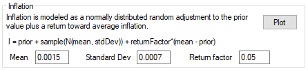 On the “Market” page you can change the values of the model inputs to see how it effects the modeled inflation. The return factor determines how strongly inflation will return to this mean value. Lower this value for more extreme swings. Standard Deviation determines how fast inflation can change.
Stock Market
The simulation doesn’t model different parts of the stock market (like small cap vs large cap or USA vs foreign), instead the simulation pretends like all your assets with the “Growth Type” set to “Stock” are invested in an S&P 500 index fund. While diversification does provide a small benefit over this assumption, the effect is small.
The simulation picks a random value for the stock market return each month. This value is truly random and is not effected by any other market variable or the previous performance of the stock market. Like with the inflation model, the random value is chosen from a distribution. Unlike the inflation model, I don’t use a normal distribution. Instead I use the Student’s t-distribution. Compared to the Normal distribution, the Student’s t has wider tails (more of the probability is on the edges). Using a Student’s t allows bigger monthly swings in the stock market. A normal distribution that matches the basic shape of historical returns makes it basically impossible to get monthly returns of +15/-11% or more. That may seem like a large monthly swing, but it has happened 8 times since 1950.
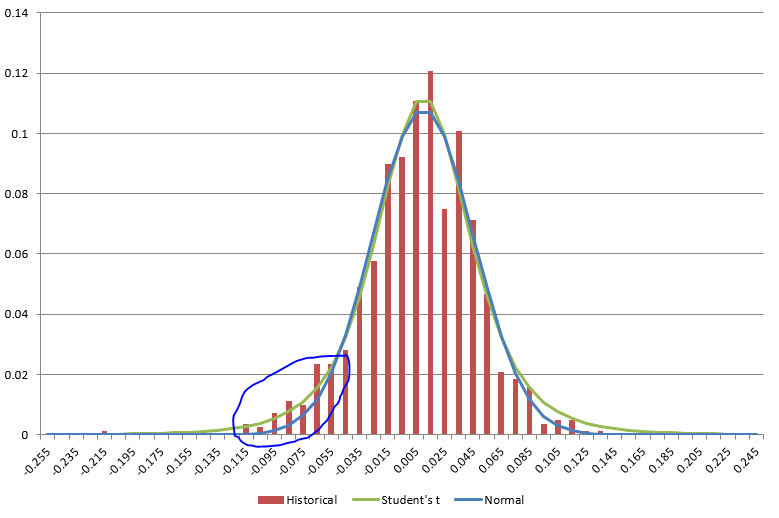 The Student’s t-distribution actually makes big swings a bit too likely, so I cap the monthly return to within -26% to +19% (historically the worst month was -22% and the best was +16%).
On the “Markets” page you can change the parameters that define the Student’s t-distribution and the min/max monthly return cap. The offset is the most important factor and determines the average monthly return. The scale and DoF determine the shape of the distribution. See the Wikipedia page for details, but increasing the DoF and lowering the scale reduces the effective variance. You can change these values and then plot the distribution curve against the historical returns.
For reference when you are trying to match historical data with your market settings: The average monthly return since 1950 is 0.7% with a standard deviation of 0.04. In the last 20 years, the monthly return has been 0.5% with a standard deviation of 0.043.
Dividends
Stocks pay dividends separately from the amount that their value changes. In a year where the stock market goes down, stocks will still pay dividends. Like inflation, dividends are fairly consistent month to month. Unlike inflation, dividend payments are correlated (negatively) with stock prices. So I model dividend yield with the following formula:
DividendYield = PriorDividend + ReturnFactor*(Mean-PriorDividend) + StockCorrelation*StockReturn
if ( DividendYield < 0 ) DividendYield = 0
The PriorDividend is the value of the DividendYield last month. ReturnFactor, Mean and StockCorrelation are variables that can be set on the “Markets” page. The StockReturn is this month’s change in the stock market. It isn’t possible to have a negative dividend, so if that were to happen, I set the yield to zero.
Like the inflation model, the Mean is the most important factor and will determine the average value of dividend yields over many runs. Historically, dividends have averaged 3.2% over the last 50 years but only 2.2% over the last 30 years.
Real Estate
I model the change in real estate prices as Inflation + 1.5%/12 each month.
I am assuming that real estate always grows 1.5% faster than inflation (yearly). This simple model is fine for situations where your real estate assets are limited to properties that you hold for many years (like your primary residence). If you are using real estate for a large portion of the assets that you use to pay expenses, this model will generate results that are too optimistic.
You can change the 1.5% on the “Data” page.
Bonds
The simulation doesn’t distinguish between different types of bonds and assumes that any assets with a “Growth Type” of “Bond” are invested in a blend of AAA and Baa bonds. If you have a significant amount of assets in junk bonds or treasury bonds, you should modify the model parameters to better match the return and uncertainty of your bonds.
Like with inflation and dividends, bond yields are fairly stable and correlated with last month’s yield. Bond yields are also somewhat correlated with inflation. The simulation models bond yields with the following formula:
BondYield = PriorYield + Random(Normal(Mean, Variance)) + ReturnFactor*(Mean-PriorYield+Inflation)
PriorYield is last month’s bond yield, Mean is the average bond yield over inflation, Variance is the variance of the distribution and Inflation is this month’s value of inflation.
The Mean, Variance and ReturnFactor can be adjusted and the yield plotted against historical values. Historically, corporate bonds have yielded 7.2% since 1950 but only 4.5% over the last 20 years. The rate above inflation has been more consistent: 3.6% since 1950 and 2.3% over the last 20 years.
Changing the defaults
Adjusting the parameters of the model can be done on the “Market” page. For each modeled variable, you can plot a simulated run and look at how it compares to the historical performance. The higher you set the standard deviations, the more times you should plot a run to get a feel for how it will perform.
For the stock market, the program also allows you to plot the student’s t-distribution against the historical monthly returns.
Even with these tools, it can be difficult to see how your changes will effect the simulation. So there is also an option to “Run 25k trials and display statistics”. This will run the full simulation 25,000 times and compile stats about what the market variables did.
For each run, the program keeps track of the min/max and average value of each variable. After all 25,000 runs, it reports the average value of the minimum and maximum values, the overall average value and the average standard deviation.
You can compare these values to historical data (or some other metric you want to match) to make sure that your settings will generate reasonable market performance.